-
 AARON DEES 14 Apr
Cross Platform
Entropy Coding
Quantization
Integer Networks
Data Compression
variational models

A review of "Integer Networks for Data Compression with Latent-Variable Models" by Aaron Dees and Myles Doyle.
TL;DR
This paper tackles the issue of the breakdown of entropy coding when the prior of a variational latent-variable model is computed on different hardware or software platforms. The solution proposed in the paper is to use ‘Integer Networks’, which attempts to remove the floating-point math that causes this non-deterministic behaviour across platforms. The results show that using such networks on both the computation of the prior as well as the representation itself can yield reliable cross-platform encoding and decoding of images using variational models. The paper highlights how an Integer Network architecture can be constructed, as well as how training can be adapted to account for this change.
Introduction
Variational latent-variable models are a popular choice for modern data compression. In short, successful variational latent-variable models can represent relevant information in the data they are trained for in a compact fashion.
Overview
A variational autoencoder (VAE) is a type of variational latent-variable model that can be used for image compression. We can break the simple deep learning compression pipeline shown in Figure 1 below into several steps:
- Encode \(\mathbf{y}\) latent:
- Given an input image \(\mathbf{x}\), generate a latent representation \(\mathbf{y}\) of an image using an encoder network
- Quantise the latent \(\mathbf{y}\) to produce \(\hat{\mathbf{y}}\)
- Encode \(\hat{\mathbf{y}}\) to a bitstream by passing the entropy parameters \(\mathbf{\mu_y}\) and \(\mathbf{\sigma_y}\) along with \(\hat{\mathbf{y}}\) to the entropy encoder to produce a bitstream for \(\hat{\mathbf{y}}\)
- Decode the bitstream for \(\hat{\mathbf{y}}\) by passing it and the entropy parameters for \(\hat{\mathbf{y}}\) (\(\mathbf{\mu_y}\) and \(\mathbf{\sigma_y}\)) to the entropy decoder to get \(\hat{\mathbf{y}}\)
- Pass \(\hat{\mathbf{y}}\) to the decoder to produce \(\hat{\mathbf{x}}\) (which hopefully looks like the original image \(\mathbf{x}\))
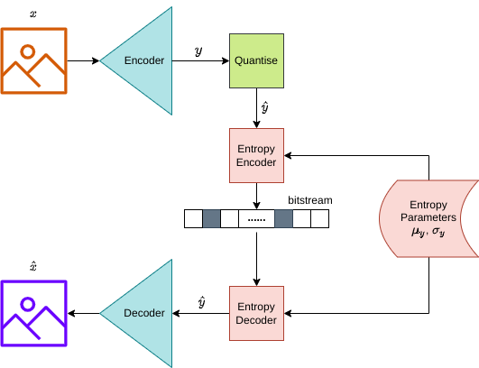 Figure 1: Simple model architecture for image compression. This model architecture describes the steps to encode and decode an image using a very simple variational model with a neural network based encoder and decider (shown in the blue tetrahedrons and labelled appropriately), an arithmetic encoder and arithmetic decoder (shown as red rectangles), a quantization module (shown as a green square), and finally a factorized entropy model (shown as a red database-rectangle with rounded edges). The diagram describes the flow of data through the pipeline to produce a bitstream for the latent \(\mathbf{y}\), followed by the decompression of the bitstream to reconstruct an image.
From the above pipeline, we define the encoder model distribution as \(e(\mathbf{y} \vert \mathbf{x})\), and the decoder model distribution as \(d(\mathbf{x} \vert \mathbf{y})\). The marginal distribution of the latent \(\mathbf{y}\) can then be written as \(m(\mathbf{y}) = \mathbb{E}_{\mathbf{x}} \left[\mathbf{y} \vert \mathbf{x} \right] \). The prior \(p(\mathbf{y})\) is a variational estimate of the marginal distribution.
The entropy parameters used by the entropy encoder and entropy decoder must be identical. This is because minor changes in these inputs can cause large changes in the entropy decoded latents. This blog will dive deeper into this issue and the solution explored in the paper.
Entropy Encoding
The universal representation of any compressed data today is the binary channel, this is restricted compared to the richness of latent representations obtained from Variational latent-variable models. Thus, for practical compression, the latent representations discussed above need to be converted to binary. This is done through entropy coding.
A popular entropy coding technique is arithmetic coding; such as range coding, or ANS coding (Duda 2014). Range coding is asymptotically optimal; in other words, the bitstream length converges to the expected KL-divergence once the representation sequence is sufficiently large. For this to hold, the sending and receiving side of the binary channel must be able to compute the prior \(p\), and have identical instances of it. In other words, it is crucial that when we encode a latent representation to a bitstream with some distribution on one communication side, we decode that bitstream with the exact same distribution on the other side. Small differences in the computation of the prior \(p\) on either side, can lead to a complete breakdown of entropy coding, leaving unreliable latent representations and thus giving garbage results, as demonstrated in Figure 2 below.
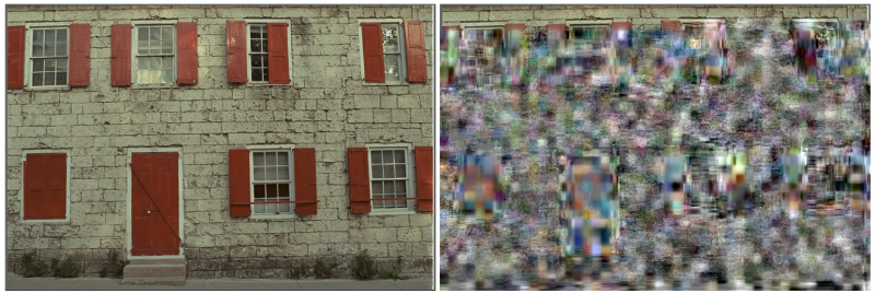 Figure 2: Left: Image decoded using integer arithmetic. Right: Image decoded using floating-point arithmetic. The image was decoded correctly, beginning in the top-left corner, until floating-point round-off error caused a small discrepancy between the sender and the receiver's computation of prior, p, at which point the error propagated catastrophically. (Ballé et al., Sept 2018)
Thus it is imperative that the computation of the prior \(p\), be identical on both sides of the binary channel.
Why would the prior differ?
In typical compression applications, the sender and receiver may be using different hardware or software platforms. This becomes an issue as floating-point math and numerical round-off are highly platform-dependent and cannot presently be made deterministic across arbitrary platforms. Therefore, performing the computation of the prior on heterogeneous platforms may not yield the same results, which as we mentioned, is required by range coding to guarantee its deterministic behaviour, else we will likely get catastrophic results similar to those in Figure 2. In some cases, it is even noted that round-off errors can be non-deterministic on the same platform (Ballé et al., Sept 2018).
Additionally, latent-variable models that employ ANNs to compute priors and other learned image compression models (Ballé et al., Feb 2018), are likely to be even more vulnerable to such issues. This is because ANNs generally use large amounts of floating-point math.
How can this issue be resolved?
The solution proposed in this paper is to use integer arithmetic. They construct a type of quantized neural network called Integer Networks, targeted at generative and compression models, to prevent cross-platform non-determinism in the computation of the prior \(p\). They also expand on this by using Integer Networks for computing the representation itself, highlighting the ability to remove any non-deterministic behaviour in the entire pipeline of learned image compression models (Ballé et al., Sept 2018).
Results
To access the efficacy of Integer Networks in enabling platform-independent compression and decompression an image compression model described in Balle et al (Feb 2018) was used, this can be seen in Figure 3, below;
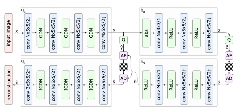 Figure 3: Image Compression Model architecture used to evaluate the efficacy of Integer Networks in enabling platform-independent compression and decompression (Ballé et al., Feb 2018)
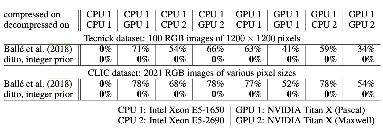
The above is a familiar model defined with a hyperprior network. The paper compares the original model seen in Figure 3, with a version in which the network \(h_s\) , used to compute the prior, is replaced with an integer network. Several experiments were run on different platform combinations to test the robustness of the model's determinism across platforms.
As seen in Table 1 below, the original model incorrectly decompresses over 50% of images on average when the pipeline is split across platforms. The modified model on the other hand reduces this failure rate to 0%.
Model performance is also tested using rate-distortion performance against bits per pixel. This can be seen in Figure 4 (left). Here, the modified model performs identically to the original which is what we would expect given the only change is to the calculation of the prior and not the latent representation itself.
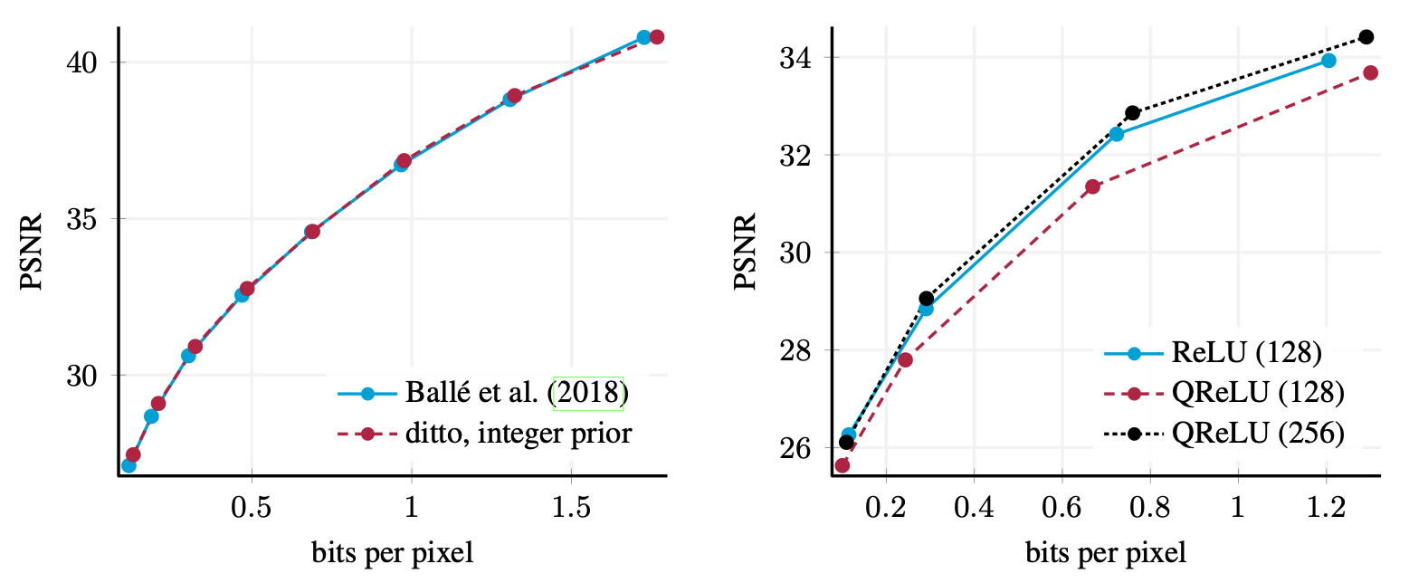 Figure 4: Rate-distortion performance of image compression models (Ballé et al., Sept 2018). Left: Performance of Ballé et al. (Feb 2018) vs the same model with integer prior. Performance is identical. Right: Performance of Ballé et al. (Feb 2018) ReLU model with 128 filters per layer vs. the same model, with integer transforms and QReLU activation functions with 128 or 256 filters per layer.
Experiments were also carried out on using Integer Networks throughout the model, using Balle's ReLU model, Ballé (July 2018). It was found that the rate-distortion performance for these decreased, as seen in Figure 4 (right). The reason highlighted for this is that decreased accuracy obtained using integer arithmetic leads to a lower approximation capacity than with floating-point networks. This loss in model performance is compensated by increasing the number of filters per layer. It is noted that this increases the training time required for model convergence, it's also noted that it may not affect runtime, as the storage overhead required for the integer implementation is lower and integer arithmetic is computationally less complex. Presumably, this is unverified.
Implementation
Integer Networks
As we've previously discussed, the paper proposes the use of Integer Networks to ensure the network is deterministic on a wide variety of platforms. It proposes restricting all data types to integers and that all operations use basic arithmetic or lookup tables. Since integer multiplications increase the output range compared to that of the input range, an additional step is required after each linear operation, where each output is scaled by a learned parameter, \(\textbf{c}\). Meaning the relationship between inputs \(\mathbf{u}\) and outputs \(\mathbf{w}\) , is as follows;
\[ \mathbf{v}=(\mathbf{H}\mathbf{u}+\mathbf{b}) \oslash \textbf{c} \]
\[ \mathbf{w} = g(\mathbf{v}) \]
Where, \(\mathbf{H}\) is some linear transform (MM or Conv), \(\mathbf{b}\) is bias vector, \(\mathbf{c}\) is the scaling parameter vector, and \(g\) is the nonlinearity. \(\oslash\) represents rounded division. All values mentioned above and all intermediate results are stored as integers, but not necessarily of the same format. An example set of number formats proposed in the paper are as follows;
\(\mathbf{H}\): 8-bit signed
\(\mathbf{b}, \mathbf{v}\): 32-bit signed
\(\mathbf{c}\): 32-bit unsigned
\(\mathbf{w}\): 8-bit unsigned
We infer from the above that the accumulators of the linear transform require a larger bit width than the activation and filter coefficients, to account for the potential increased output range due to multiplicative operations. This means that \(\mathbf{b}, \mathbf{v}, \mathbf{c}\) also require this same bit width. The paper also proposes that the nonlinearity \(g\), can be implemented with a simple clipping operation, as follows;
\[g_{QReLU}(\mathbf{v}) = \max\left( \min\left( \mathbf{v}, 255\right), 0\right).\]
Training Integer Networks
The paper also suggests some solutions to overcome training difficulties. It proposes that the network is trained entirely using floating point computations, rounding to integers after every computation, with back propagation done entirely in floating point precision. Integer parameters, \(\mathbf{H}\), \(\mathbf{b}\) and \(\mathbf{c}\) are defined as functions of their floating point equivalents, \(\mathbf{H'}\), \(\mathbf{b'}\) and \(\mathbf{c'}\), respectively;
\[\mathbf{H'} = \begin{bmatrix} Q\left( \mathbf{h'_{1}} / s\left( \mathbf{h'_{1}} \right) \right) \\ \vdots \\ Q\left( \mathbf{h'_{N}} / s\left( \mathbf{h'_{N}} \right) \right)\end{bmatrix} ,\]
\[\mathbf{b}=Q\left(2^K \mathbf{b'} \right),\]
\[ \mathbf{c} = Q \left( 2^{K} r \left( \mathbf{c'} \right) \right) ,\]
where \(Q\) is an operator which rounds to the nearest integer, and \(\mathbf{b'}\) and \(\mathbf{c'}\) are scaled by the bit width of the kernel \(K\). In the previous example this was 8 bits. When \(\mathbf{c}\) is small there can be fluctuations in the quotient and thus the input to the nonlinearity which can lead to instability in training, to tackle this the reparameterization mapping \(r\) is used from Ballé (July 2018);
\[r(c') = \max\left( c', \sqrt{1+\epsilon^2}\right)^2 - \epsilon^2,\]
where \(\epsilon\) is a small constant. Essentially, this prevents parameters both getting 'stuck' at zero, and/or having negative values. In training the step size \(\mathbf{c}\) is multiplied with a factor that's approximately linear in \(\mathbf{c}\), meaning that \(r\) ensures that \(\mathbf{c} > 0\), while gracefully scaling down gradients on \(\mathbf{c}\) close to zero.
To ensure that \(\mathbf{H}\) fills the dynamic range bound, \((-2^{K-1}, 2^{K-1}]\) (while keeping zero values at zero), a rescaling factor is also applied before the rounding each element of, \(\mathbf{H'}\);
\[s\left(\mathbf{h'} \right) = \max \left( \left(-2^{K-1}\right)^{-1} \min_i h_i' , \left(2^{K-1} - 1\right) ^{-1} \max_i h_i', \epsilon \right).\]
A small constant is used, for example, \(\epsilon=10^{-20}\), to replace zero values to ensure there is no division of zero.
As you'd expect an issue occurs when trying to backpropagate gradients into these parameters as rounding has zero gradients almost everywhere. The workaround for this highlighted in the paper is to replace the derivative of such rounding functions with an identity function.
Derivatives of the loss functions are computed wrt \(\mathbf{H'}\), \(\mathbf{b'}\) and \(\mathbf{c'}\), assuming the following;
\[ \frac{\partial \mathbf{h}}{\partial \mathbf{h'}} := \frac{1}{s \left( \mathbf{h'} \right)}, \quad \frac{\partial \mathbf{b}}{\partial \mathbf{b'}} := 2^{K}, \quad \frac{\partial \mathbf{c}}{\partial \mathbf{c'}} := 2^K r'\left( \mathbf{c'} \right), \]
where \(s\) is treated as a constant, and \(r'\) is the replacement gradient function proposed by Ballé (July 2018). Here it is proposed to either use projected gradient descent, alternating between a descent step on \(c'\) with \(r(c')=c'^2 - \epsilon^2\) and a projection step with \(c'=\max\left( c', \sqrt{1+\epsilon^2}\right)\), or by performing gradient descent directly on the reformulation, \(r(c')\). This involves replacing the gradient of the maximum operation \(m = \max(c', v)\) with respect to the loss function \(L\);
\[ \frac{\partial L}{\partial c'} = \frac{\partial L}{\partial m} \frac{\partial m}{\partial c'} := \begin{cases} \frac{\partial L}{\partial m}&{c' \geq v \text{ or } \frac{\partial L}{\partial m} < 0} \\ 0&\text{otherwise} \end{cases}\]
Where \(v = \sqrt{1+\epsilon^2}\), meaning this propagates updates to \(c'\) even when it is smaller than \(v\).
Once training is completed, integer parameters \(\mathbf{H}\), \(\mathbf{b}\) and \(\mathbf{c}\) are computed once more. These are the parameters used for evaluation.
On top of rounding parameters, it is also required to round the activations. To get gradients for rounding division \(\oslash\), it is suggested to substitute the gradient for standard floating-point division. To estimate gradients for the rounding activation functions it is proposed that the gradient is replaced with the corresponding non-rounded activation function. The paper highlights issues that can lead to training getting stuck when calculating gradients for the Quantised ReLU (QReLU). It offers a solution by replacing the gradient of \( \frac{\partial g_{QReLU} \left(v\right) }{\partial \mathbf{v}} \). For further details on this please see Ballé et al. (Sep 2018).
Computing the Prior with Integer Networks
Assuming the prior on the latent representation if given by \(p(\mathbf{y} | \mathbf{z})\) and that \(p\) is a known distribution, with parameters \(\theta_i\) computed by some neural network \(g\). Then
\[ p\left( \mathbf{y} \mid \mathbf{z} \right) = \prod\limits_i p\left( y_i \mid \mathbf{y}_{:i}, \mathbf{z} \right). \]
where \(\mathbf{y}_{:i}\) denotes the vector consisting of all elements before the \(i\)th element. It is proposed that \(g\) can be computed deterministically using Integer Networks, by discretizing the parameters \(\theta\) to a reasonable accuracy, using a simple reformulation of the scale parameters obtained from \(g\). An example distribution of a modified Gaussian with scale parameters conditioned on a latent variable is used as per Ballé et al. (Feb 2018);
\[ p\left( \mathbf{y} \mid \mathbf{z} \right) = \prod\limits_i \left( \mathcal{N}\left(0,\sigma_i^2\right) \mathcal{U}\left(-\frac{1}{2}, \frac{1}{2} \right) \right)\left(y_i\right)\]
with \(\mathbf{\sigma} = g\left(\mathbf{z}\right)\). With the scale parameters, \(sigma\) reformulated as follows;
\[ \sigma_i = \exp\left( \log\left( \sigma_{\min}\right) + \frac{\log\left(\sigma_{\max}\right) - \log \left(\sigma_{\min}\right)}{L-1} \theta_i \right), \]
where \(\theta = g\left(\mathbf{z}\right) \) is computed usig the integer network. The final activation in \( g \) is chosen such that the integer outputs have \(L\) levels in the range \(\left[0,L-1 \right]\).
Computing the Representation with Integer Networks
Now that we have a well-defined method of training our network using an integer network, and have identical priors used in encoding and decoding of the bitstream, how can we compute the latent representation of our data deterministically at validation while ensuring the marginal resembles a smooth function during training?
To do this the model must be robust to non-determinism both in training and at validation. This has been explored for categorical distributions and vector-quantization by Jang et all. (2017) and Agustsson et al. (2017) respectively. They evaluate their ANNs followed by an argmax to get some deterministic output while using softmax with rounded inputs instead during training to get useful gradients. This allows for a platform-independent pipeline.
As we are familiar with, from previous work by Ballé et al. (Feb 2018) probabilistic encoder distributions are used for training which is replaced with a deterministic probabilistic encoder during evaluation. The probabilistic encoder distribution used in training is
\[e\left(\mathbf{y} \middle| \mathbf{x} \right) = \mathcal{U}\left(\mathbf{y} \middle| g\left(\mathbf{x}\right) - \frac{1}{2}, g\left(\mathbf{x}\right) + \frac{1}{2}\right),\]
where \(\mathcal{U}\) is the uniform distribution and \(g\) is an ANN. This makes \(\mathbf{y}\) shift invariant. Choosing \(\mathbf{o}\) as a sub-integer offset such that the mode or median of the distribution \(e\left(\mathbf{y} \middle| \mathbf{x} \right) \) is centered on one of the quantization bins. Furthermore, if \(g\) is an integer ANN, the previous equation becomes equivalent to the following;
\[e\left(\mathbf{y} \middle| \mathbf{x} \right) = \mathcal{U}\left(\mathbf{y} \middle| Q\left(g\left(\mathbf{x}\right)\right) - \frac{1}{2}, Q\left(g\left(\mathbf{x}\right)\right) + \frac{1}{2}\right),\]
since \(g\) computes integer outputs, which is equivalent to quantization.
Training with the above construction was found to lead to instabilities. These were potentially caused by the marginal \( m \left(\mathbf{y}\right) = E_\mathbf{x} \left( e\left( \mathbf{y} \middle| \mathbf{x} \right) \right) \) resembling a piecewise constant function, while the prior must be forced to be smooth, else no useful gradients would be obtained by \( E_\mathbf{x} \left( D_{KL} [ e \middle| \middle| p ] \right) \).
As a solution to this issue, the paper proposes using the first of the two equations above during training, but with the last layer of \( g\) having no non-linearity and using floating point division instead of integer division. Given input \(\mathbf{u}\) as the input to the last layer in \(g\), this gives;
\[e\left(\mathbf{y} \middle| \mathbf{x} \right) = \mathcal{U}\left(\mathbf{y} \middle| \left( \mathbf{Hu} + \mathbf{b} \right)/ \mathbf{c} - \frac{1}{2}, \left( \mathbf{Hu} + \mathbf{b} \right)/ \mathbf{c} + \frac{1}{2}\right),\]
where \( / \) represents elementwise floating point division. This equation is used during training. The following integer arithmetic form of this equation is used during evaluation;
\[ \mathbf{y} = \left( \mathbf{Hu} + \mathbf{b} - Q\left( \mathbf{o} \odot \mathbf{c} \right) \right) \oslash \mathbf{c}, \]
where \(\odot\) represents elementwise multiplication. It is noted that the rounded product can be folded into the bias term as a small optimization.
Now, we have a formalism where the marginal resembles a smooth function during training but can be represented deterministically during evaluation. This removes the need for regularizing the prior.
Conclusion
The paper details the formalism to define an Integer Network as well as how it differs during training and evaluation. The solution proposed in the paper clearly resolves the issue of non-determinism across training and evaluation across heterogeneous compute systems when implementing a compression pipeline. This is demonstrated in the results.
In this paper, there are two techniques explored that are very interesting:
- the use of Integer Networks to invoke determinism across different compute architectures
- that the priors are obtained using a discretized CDF
References
Ágústsson, E.Þ. et al., n.d. Soft-to-Hard Vector Quantization for End-to-End Learning Compressible Representations. Advances in Neural Information Processing Systems 30, 1141–1151.
Ballé, J., July 2018. Efficient Nonlinear Transforms for Lossy Image Compression. arXiv:1802.00847 [eess].
Ballé, J., Johnston, N., Minnen, D., Sept 2018a. Integer Networks for Data Compression with Latent-Variable Models. Presented at the International Conference on Learning Representations.
Ballé, J., Minnen, D., Singh, S., Hwang, S.J., Johnston, N., Jan 2018b. Variational image compression with a scale hyperprior. Presented at the International Conference on Learning Representations.
Duda, J., 2014. Asymmetric numeral systems: entropy coding combining speed of Huffman coding with compression rate of arithmetic coding. arXiv:1311.2540 [cs, math].
Jang, E., Gu, S., Poole, B., 2016. Categorical Reparameterization with Gumbel-Softmax.
RELATED BLOGS
 ARSALAN ZAFAR
- 22 Apr
 BILAL ABBASI
- 14 Apr
 HAMZA ALAWIYE
- 11 Oct


